Overview
This vignette describes how to install the package ‘PINstimation’, either in its stable version on CRAN, or in its development version of Github. It also provides several usage examples on how to use the different functionalities of the package.
Installation
The easiest way to get PINstimation is the following:
install.packages("PINstimation")To get a bug fix or to use a feature from the development version, you can install the development version of PINstimation from GitHub.
# install.packages("devtools")
# library(devtools)
devtools::install_github("monty-se/PINstimation")
Loading the package
Note to frequent users
If you are a frequent user of PINstimation, you might want to avoid repetitively loading the package PINstimation whenever you open a new R session. You can do that by adding PINstimation to .R profile either manually, or using the function load_pinstimation_for_good().
To automatically load PINstimation, run load_pinstimation_for_good(), and the following code will be added to your .R profile.
if (interactive()) suppressMessages(require(PINstimation))After restart of the R session, PINstimation will be loaded automatically, whenever a new R session is started. To remove the automatic loading of PINstimation, just open the .R profile for editing usethis::edit_r_profile(), find the code above, and delete it.
Usage examples
Below, you find five usage examples for the main functions in the package.
Example 1: [PIN] Use daily trade data to estimate the standard probability of informed trading.
Example 2: [MPIN] Use daily trade data to estimate the number of layers in the data, as well as the multi-layer probability of informed trading.
Example 3: [AdjPIN] Use daily trade data to estimate the adjusted probability of informed trading.
Example 4: [VPIN] Use high-frequency data to estimate the volume-adjusted probability of informed trading.
Example 5: Classify high frequency trades into daily trading data, and use it to estimate the adjusted probability of informed trading using the Maximum-likelihood method, and the Expectation-Maximization algorithm.
Example 1: Estimate the PIN model
We estimate the PIN model on preloaded dataset dailytrades using the initial parameter sets of Ersan & Alici (2006).
estimate <- pin_ea(dailytrades)## [+] PIN Estimation started
## |[1] Likelihood function factorization: Ersan (2016)
## |[2] Loading initial parameter sets : 5 EA initial set(s) loaded
## |[3] Estimating PIN model (1996) : Using Maximum Likelihood Estimation
## |+++++++++++++++++++++++++++++++++++++| 100% of PIN estimation completed
## [+] PIN Estimation completed
show(estimate)## ----------------------------------
## PIN estimation completed successfully
## ----------------------------------
## Initial parameter sets : Ersan and Alici (2016)
## Likelihood factorization: Ersan (2016)
## ----------------------------------
## 5 initial set(s) are used in the estimation
## Type object@initialsets to see the initial parameter sets used
##
## PIN model
##
## ========== ===========
## Variables Estimates
## ========== ===========
## alpha 0.749997
## delta 0.133334
## mu 1193.52
## eps.b 357.27
## eps.s 328.63
## ----
## Likelihood (3226.469)
## PIN 0.566172
## ========== ===========
##
## -------
## Running time: 1.53 secondsExample 2: Estimate the Multilayer PIN model
We run the estimation of the MPIN model on preloaded dataset dailytrades using:
- the maximum-likelihood method.
ml_estimate <- mpin_ml(dailytrades)## [+] MPIN estimation started
## |[1] Detecting layers from data : using Ersan and Ghachem (2022a)
## |[=] Number of layers in the data : 3 information layer(s) detected
## |[2] Computing initial parameter sets : using algorithm of Ersan (2016)
## |[3] Estimating the MPIN model : Maximum-likelihood standard estimation
## |+++++++++++++++++++++++++++++++++++++| 100% of mpin estimation completed
## [+] MPIN estimation completed- the ECM algorithm.
ecm_estimate <- mpin_ecm(dailytrades)## [+] MPIN estimation started
## |[1] Computing the range of layers : information layers from 1 to 8
## |[2] Computing initial parameter sets : using algorithm of Ersan (2016)
## |[=] Selecting initial parameter sets : max 100 initial sets per estimation
## |[3] Estimating the MPIN model : Expectation-Conditional Maximization algorithm
## |+++++++++++++++++++++++++++++++++++++| 100% of estimation completed [8 layer(s)]
## |[3] Selecting the optimal model : using lowest Information Criterion (BIC)
## [+] MPIN estimation completedCompare the aggregate parameters obtained from the ML, and ECM estimations.
mpin_comparison <- rbind(ml_estimate@aggregates, ecm_estimate@aggregates)
rownames(mpin_comparison) <- c("ML", "ECM")
## Probabilities of ML, and ECM estimations of the MPIN model## alpha delta mu eps.b eps.s
## ML 0.750004 0.1333320 1210.984 336.9118 335.8871
## ECM 0.750000 0.1333333 1211.001 336.9052 335.8866Display the summary of the model estimates for all number of layers.
summary <- getSummary(ecm_estimate)## layers em.layers MPIN Likelihood AIC BIC AWE
## Model[1] 1 1 0.566 -3226.469 6462.9 6473.4 6508.9
## Model[2] 2 2 0.577 -800.379 1616.8 1633.5 1690.3
## Model[3] 3 3 0.574 -643.458 1308.9 1332.0 1410.0
## Model[4] 4 3 0.574 -643.458 1308.9 1332.0 1410.0
## Model[5] 5 3 0.574 -643.458 1308.9 1332.0 1410.0
## Model[6] 6 3 0.574 -643.458 1308.9 1332.0 1410.0
## Model[7] 7 4 0.575 -642.631 1313.3 1342.6 1441.9
## Model[8] 8 4 0.575 -642.631 1313.3 1342.6 1441.9Example 3: Estimate the Adjusted PIN model
We estimate the adjusted PIN model on preloaded dataset dailytrades using 20 initial parameter sets computed by the algorithm of Ersan and Ghachem (2022b).
estimate_adjpin <- adjpin(dailytrades, method = "ML", initialsets = "GE")## [+] AdjPIN estimation started
## |[1] Computing initial parameter sets : 20 GE initial sets generated
## |[2] Estimating the AdjPIN model : Maximum-likelihood Standard Estimation
## |+++++++++++++++++++++++++++++++++++++| 100% of AdjPIN estimation completed
## [+] AdjPIN estimation completed
show(estimate_adjpin)## ----------------------------------
## AdjPIN estimation completed successfully
## ----------------------------------
## Likelihood factorization: Ersan and Ghachem (2022b)
## Estimation Algorithm : Maximum Likelihood Estimation
## Initial parameter sets : Ersan and Ghachem (2022b)
## Model Restrictions : Unrestricted model
## ----------------------------------
## 20 initial set(s) are used in the estimation
## Type object@initialsets to see the initial parameter sets used
##
## AdjPIN model
##
## =========== ==============
## Variables Estimates
## =========== ==============
## alpha 0.618052
## delta 0.113091
## theta 0.090843
## theta' 0.633865
## ----
## eps.b 336.87
## eps.s 334.24
## mu.b 602.25
## mu.s 876.07
## d.b 910.98
## d.s 3.69
## ----
## Likelihood (896.427)
## adjPIN 0.269434
## PSOS 0.268542
## =========== ==============
##
## -------
## Running time: 12.667 secondsExample 4: Estimate the Volume-adjusted PIN model
We run a VPIN estimation on preloaded dataset hfdata with timebarsize of 5 minutes (300 seconds).
estimate.vpin <- vpin(hfdata, timebarsize = 300)## [+] VPIN Estimation started.
## |-[1] Checking and preparing the data...
## |-[2] Creating 300-second timebars...
## |-[3] Calculating Volume Bucket Size (VBS) and Sigma(DP)...
## |-[4] Breaking up large 300-second timebars' volume...
## |-[5] Assigning 300-second timebars into buckets...
## |-[6] Balancing timebars and adjusting bucket sizes to VBS...
## |-[7] Calculating aggregate bucket data...
## |-[8] Calculating VPIN vector...
## [+] VPIN estimation completed
show(estimate.vpin)## ----------------------------------
## VPIN estimation completed successfully.
## ----------------------------------
## Type object@vpin to access the VPIN vector.
## Type object@bucketdata to access data used to construct the VPIN vector.
## Type object@dailyvpin to access the daily VPIN vectors.
##
## [+] VPIN descriptive statistics
##
## | | Min. | 1st Qu. | Median | Mean | 3rd Qu. | Max. | NA's |
## |:-----|:-----:|:-------:|:------:|:-----:|:-------:|:-----:|:----:|
## |value | 0.101 | 0.185 | 0.238 | 0.244 | 0.29 | 0.636 | 49 |
##
##
## [+] VPIN parameters
##
## | tbSize | buckets | samplength | VBS | #days |
## |:------:|:-------:|:----------:|:--------:|:-----:|
## | 300 | 50 | 50 | 36321.25 | 77 |
##
## -------
## Running time: 3.753 secondsPlot the unweighted daily vpin stored at the variable dvpin in the dataframe dailyvpin stored at the slot @dailyvpin of the object estimate.vpin.
plot(estimate.vpin@dailyvpin$dvpin ~seq_len(nrow(estimate.vpin@dailyvpin)),
     lwd=1 , type="l" , bty="n" , xlab="day" , ylab="daily vpin",
     col=rgb(0.2,0.4,0.6,0.8) )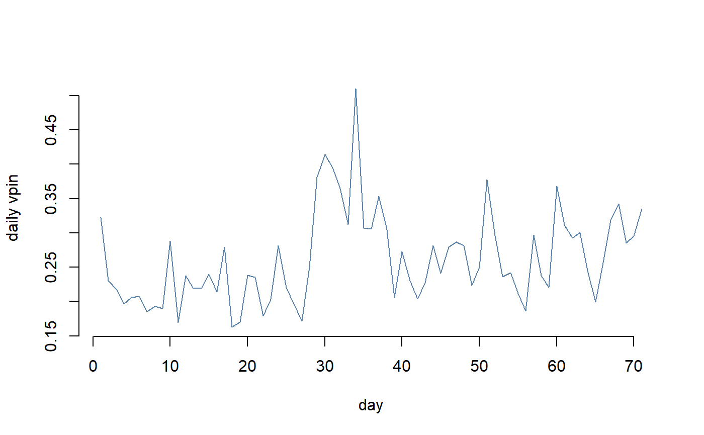
Example 5: Estimate the AdjPIN model using aggregated high-frequency data
We use the preloaded high-frequency dataset hfdata, prepare it for aggregation, and then extract 500 000 trades.
data <- hfdata
data$volume <- NULL
We classify data using the LR algorithm with a time lag of 500 milliseconds (0.5 s), using the function aggregate_data().
daytrades <- aggregate_trades(data, algorithm = "LR", timelag = 500)## [+] Trade classification started
## |[=] Classification algorithm : LR algorithm
## |[=] Number of trades in dataset : 100 000 trades
## |[=] Time lag of lagged variables : 500 milliseconds
## |[1] Computing lagged variables : using parallel processing
## |+++++++++++++++++++++++++++++++++++++| 100% of variables computed
## |[=] Computed lagged variables : in 7.68 seconds
## |[2] Computing aggregated trades : using lagged variables
## [+] Trade classification completed We use the obtained dataset to estimate the (adjusted) probability of informed trading via the two available estimated methods, i.e, the standard Maximum-likelihood method, and the Expectation-Maximization algorithm.
adjpin_ml <- adjpin(daytrades, method = "ML", initialsets = "GE")## [+] AdjPIN estimation started
## |[1] Computing initial parameter sets : 20 GE initial sets generated
## |[2] Estimating the AdjPIN model : Maximum-likelihood Standard Estimation
## |+++++++++++++++++++++++++++++++++++++| 100% of AdjPIN estimation completed
## [+] AdjPIN estimation completed
adjpin_ecm <- adjpin(daytrades, method = "ECM", initialsets = "GE")## [+] AdjPIN estimation started
## |[1] Computing initial parameter sets : 20 GE initial sets generated
## |[2] Estimating the AdjPIN model : Expectation-Conditional Maximization algorithm
## |+++++++++++++++++++++++++++++++++++++| 100% of AdjPIN estimation completed
## [+] AdjPIN estimation completedCompare the estimated parameters obtained from the ML, and ECM parameters.
adj.prob <- rbind(adjpin_ml@parameters[1:4], adjpin_ecm@parameters[1:4])
rownames(adj.prob) <- c("ML", "ECM")
## Probabilities of ML, and ECM estimations of the AdjPIN model## alpha delta theta thetap
## ML 0.5925374 0.1511567 0.3597389 0.9999995
## ECM 0.5925419 0.1512520 0.3597634 1.0000000
adj.params <- rbind(adjpin_ml@parameters[5:10], adjpin_ecm@parameters[5:10])
rownames(adj.params) <- c("ML", "ECM")
## Rate parameters of ML and ECM estimations of the AdjPIN model## eps.b eps.s mu.b mu.s d.b d.s
## ML 549.8239 546.3564 47.76120 71.67589 212.7528 223.7200
## ECM 549.8333 546.3333 47.76279 71.76036 212.7464 223.7497Getting help
If you encounter a clear bug, please file an issue with a minimal reproducible example on GitHub.